
今回は、以下のNVIDIAの実験の記事にインスパイアされた取り組みになります。
上記の記事では、NVIDIAが提案した深層学習モデルPilotNetを使った実験が紹介されています。
PilotNetは、自動運転車の運転判断をサポートするための深層学習モデルです。
車載カメラの画像を入力し、それに基づいてEnd2Endで運転操作(例えば、ステアリング操作)を出力するモデルです。
さらに記事では、そのようにして学習されたPilotNetは、運転操作を出力するために画像のどの部分を注視しているのかといった判断根拠を可視化する試みも行っています。
今回は、自動運転向けに収集・公開されたデータセットを使って同様の実験を試してみます。
データセットの準備
PilotNetを実装する上で、まずは自動運転のための画像とステアリング操作のデータセットを準備します。
今回の実装では、以下のUdacityが提供する自動運転車のデータセットを使用します。
データセットには、実際の道路環境での運転時の画像とセンサーデータが記録されており、学習に適していそうです。
実際にデータの中身を確認してみて、今回使うカラムに限定すると以下のようなデータセットになっています。
import functools
import numpy as np
import pandas as pd
import matplotlib
import matplotlib.pyplot as plt
from PIL import Image

target_output_path = './udacity-driving-reader/legacy_data_sunny/output/'

df_camera = pd.read_csv(target_output_path + 'camera.csv')
df_steering = pd.read_csv(target_output_path + 'steering.csv')

df_camera = df_camera[df_camera['frame_id'] == 'center_camera']
df_camera['timestamp'] = pd.to_datetime(df_camera['timestamp'])
df_camera.set_index(['timestamp'], inplace=True)
df_camera.index.rename('index', inplace=True)

df_steering['timestamp'] = pd.to_datetime(df_steering['timestamp'])
df_steering.set_index(['timestamp'], inplace=True)
df_steering.index.rename('index', inplace=True)

df_merged = functools.reduce(lambda left, right: pd.merge(left, right, how='outer', left_index=True, right_index=True), [df_camera, df_steering])
df_merged.interpolate(method='time', inplace=True)
df_filtered = df_merged.loc[df_camera.index]
df_filtered.fillna(0.0, inplace=True)
df_filtered.index.rename('timestamp', inplace=True)
df_filtered = df_filtered.reset_index()
df_filtered = df_filtered[['timestamp', 'filename', 'angle', 'speed']]
df_filtered['filename'] = target_output_path + df_filtered['filename']

# 停止している画像・不自然にハンドルが切れすぎている画像を除き、正規化
df_filtered = df_filtered[10 < df_filtered['speed']]
df_filtered = df_filtered[(-0.5 <= df_filtered['angle']) & (df_filtered['angle'] <= 0.5)]
df_filtered['angle'] += 0.5
df_filtered = df_filtered.sample(frac=1)

df_filtered.head()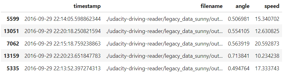
データセットには画像パスが格納されていますので、何枚か画像を表示してみると以下のような感じです。
df = df_filtered.sample(frac=1)[:3]

fig, axs = plt.subplots(ncols=3, figsize=(15, 4))

for i, (index, row) in enumerate(df.iterrows()):
    img = Image.open(row['filename'])
    axs[i].imshow(img)
    axs[i].set_title('steering: {}'.format(row['angle']))

plt.show()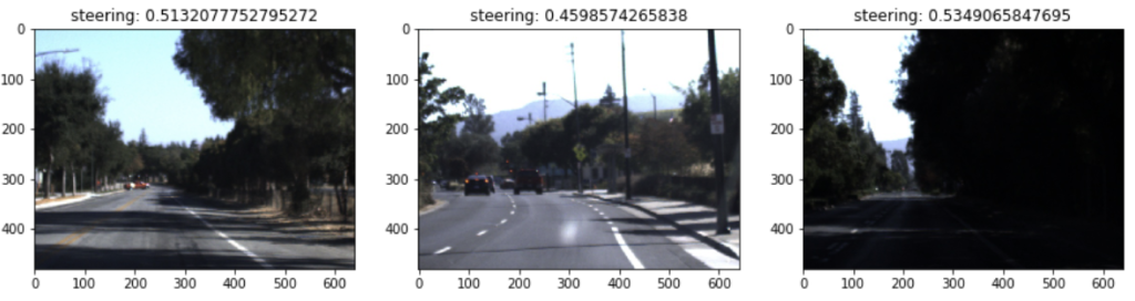
PilotNetについて
冒頭で述べました通り、PilotNetは、NVIDIAが提案するディープラーニングモデルで、自動運転車の運転判断をサポートするために設計されました。
このモデルは、カメラからの入力画像を受け取り、それに基づいて運転指示(例: ハンドルの角度)を出力します。
論文は以下です。
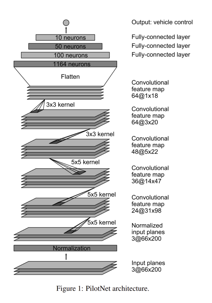
PilotNetのアーキテクチャは、畳み込みニューラルネットワーク(CNN)をベースにしています。
このネットワークは、複数の畳み込み層、活性化関数、および全結合層から構成されています。
以下は論文から抜粋のアーキテクチャ図です。
モデルの実装は以下の通りです。
深層学習のライブラリはchainerを使用しました。
class PilotNet(chainer.Chain):

    def __init__(self):
        super(PilotNet, self).__init__()
        with self.init_scope():
            self.bn0 = L.BatchNormalization(3)
            self.conv1 = L.Convolution2D(3, 24, ksize=5, stride=2)
            self.conv2 = L.Convolution2D(24, 36, ksize=5, stride=2)
            self.conv3 = L.Convolution2D(36, 48, ksize=5, stride=2)
            self.conv4 = L.Convolution2D(48, 64, ksize=3)
            self.conv5 = L.Convolution2D(64, 64, ksize=3)
            self.fc6 = L.Linear(None, 100)
            self.fc7 = L.Linear(100, 50)
            self.fc8 = L.Linear(50, 10)
            self.fc9 = L.Linear(10, 1)

    def __call__(self, x, extract_feature=False):
        h0 = self.bn0(x)
        h1 = F.relu(self.conv1(h0))
        h2 = F.relu(self.conv2(h1))
        h3 = F.relu(self.conv3(h2))
        h4 = F.relu(self.conv4(h3))
        h5 = F.relu(self.conv5(h4))
        h6 = F.dropout(F.relu(self.fc6(h5)), ratio=0.1)
        h7 = F.dropout(F.relu(self.fc7(h6)), ratio=0.1)
        h8 = F.dropout(F.relu(self.fc8(h7)), ratio=0.1)
        y = self.fc9(h8)

        if extract_feature:
            return {'conv1': h1, 'conv2': h2, 'conv3': h3, 'conv4': h4, 'conv5': h5, 'fc6': h6, 'fc7': h7, 'fc8': h8, 'fc9': y}

        return y

    def get_mask(self, x):
        h0 = self.bn0(x)
        h1 = F.relu(self.conv1(h0))
        h2 = F.relu(self.conv2(h1))
        h3 = F.relu(self.conv3(h2))
        h4 = F.relu(self.conv4(h3))
        h5 = F.relu(self.conv5(h4))

        h5 = F.mean(h5, axis=1)
        h5 = F.reshape(h5, (h5.data.shape[0], 1, h5.data.shape[1], h5.data.shape[2]))
        h5 = chainer.cuda.to_cpu(h5.data)
        h4_rev = L.Deconvolution2D(1, 1, ksize=3,
                                 initialW=np.ones((1, 1, 3, 3), dtype=np.float32),
                                 initial_bias=np.zeros((1), dtype=np.float32))(h5)
        h4 = F.mean(h4, axis=1)
        h4 = F.reshape(h4, (h4.data.shape[0], 1, h4.data.shape[1], h4.data.shape[2]))
        h4 = chainer.cuda.to_cpu(h4.data)
        h3_rev = L.Deconvolution2D(1, 1, ksize=3,
                                  initialW=np.ones((1, 1, 3, 3), dtype=np.float32),
                                  initial_bias=np.zeros((1), dtype=np.float32))(h4_rev*h4)
        h3 = F.mean(h3, axis=1)
        h3 = F.reshape(h3, (h3.data.shape[0], 1, h3.data.shape[1], h3.data.shape[2]))
        h3 = chainer.cuda.to_cpu(h3.data)
        h2_rev = L.Deconvolution2D(1, 1, ksize=5, stride=2, outsize=(h2.data.shape[2], h2.data.shape[3]),
                                  initialW=np.ones((1, 1, 5, 5), dtype=np.float32),
                                  initial_bias=np.zeros((1), dtype=np.float32))(h3_rev*h3)
        h2 = F.mean(h2, axis=1)
        h2 = F.reshape(h2, (h2.data.shape[0], 1, h2.data.shape[1], h2.data.shape[2]))
        h2 = chainer.cuda.to_cpu(h2.data)
        h1_rev = L.Deconvolution2D(1, 1, ksize=5, stride=2, outsize=(h1.data.shape[2], h1.data.shape[3]),
                                  initialW=np.ones((1, 1, 5, 5), dtype=np.float32),
                                  initial_bias=np.zeros((1), dtype=np.float32))(h2_rev*h2)
        h1 = F.mean(h1, axis=1)
        h1 = F.reshape(h1, (h1.data.shape[0], 1, h1.data.shape[1], h1.data.shape[2]))
        h1 = chainer.cuda.to_cpu(h1.data)
        mask = L.Deconvolution2D(1, 1, ksize=5, stride=2, outsize=(h0.data.shape[2], h0.data.shape[3]),
                                initialW=np.ones((1, 1, 5, 5), dtype=np.float32),
                                initial_bias=np.zeros((1), dtype=np.float32))(h1_rev*h1)

        return mask
モデルのトレーニングには、先ほどの「データセットの準備」で取得したUdacityのデータセットを使用します。
したがって、入力は車載画像で出力値はステアリング(ハンドル)の角度です。
学習のコードは以下の通り。
model = L.Classifier(PilotNet(), lossfun=F.mean_squared_error)
model.compute_accuracy = False
optimizer = chainer.optimizers.Adam(alpha=1e-4)
optimizer.setup(model)

if gpu >= 0:
    chainer.cuda.get_device(gpu).use()
    model.to_gpu(gpu)

epoch_num = 100
batch_size = 1000

train_iter = chainer.iterators.SerialIterator(train_dataset, batch_size)
test_iter = chainer.iterators.SerialIterator(valid_dataset, batch_size, repeat=False, shuffle=False)
updater = chainer.training.StandardUpdater(train_iter, optimizer, device=gpu)
trainer = chainer.training.Trainer(updater, (epoch_num, 'epoch'), out='result_pilotnet')
trainer.extend(extensions.Evaluator(test_iter, model, device=gpu))
trainer.extend(extensions.LogReport(trigger=(10, 'epoch')))
trainer.extend(extensions.LogReport())
trainer.extend(extensions.PrintReport(['epoch', 'main/loss', 'validation/main/loss', 'elapsed_time']))
trainer.extend(extensions.PlotReport(['main/loss', 'validation/main/loss'], 'epoch', file_name='loss.png'))
trainer.extend(extensions.snapshot(filename='snapshot_epoch_{.updater.epoch}.npz'), trigger=(epoch_num, 'epoch'))
trainer.run()
epoch main/loss validation/main/loss elapsed_time
10 0.0309514 0.0388316 82.0616
20 0.0122537 0.00430815 149.306
30 0.00964154 0.00319876 216.603
40 0.0084587 0.00268209 284.642
50 0.00782145 0.0022793 351.935
60 0.00739421 0.00230404 419.19
70 0.00697377 0.00171783 487.325
80 0.00672234 0.00163945 554.637
90 0.00637599 0.00138362 622.032
100 0.00623202 0.00120607 690.019 Image.open('result_pilotnet/loss.png')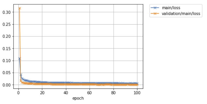
問題なく学習させることができました。
Visual Backpropagationによるステアリング操作要因の可視化
NVIDIAの記事では、PilotNetの判断を明確に理解するための方法として、Backpropagationを用いた可視化を試しています。
Backpropagationは通常、ニューラルネットワークの学習時に誤差を逆伝播させるための手法として知られていますが、この技術を利用して、モデルの出力から入力層に向かって、各ニューロンの活性化の影響度を計算することで、モデルが最終的な判断を下す際にどの入力情報を重視したのかを明らかにすることも可能です。
これにより、入力画像のどの部分がモデルの判断に大きく寄与しているのかを特定することができます。
実際にやってみると以下のようになりました。
from sklearn.preprocessing import MinMaxScaler
from PIL import ImageEnhance

col_num = 5
for i, (x, y) in enumerate(zip(valid_x, valid_y)):

    if i >= 30:
        break
    if i % col_num == 0:
        fig, axs = plt.subplots(ncols=col_num, figsize=(20, 4))

    img = Image.open(x)

    x = processing_x(img)
    x = x[np.newaxis]

    mask = model.predictor.get_mask(x)
    mask = MinMaxScaler().fit_transform(mask.data.squeeze())

    w, h = img.size
    mask *= 255
    mask = Image.fromarray(mask).convert('L')
    mask = mask.resize((((w//8)*7 - (w//8)*1), ((h//8)*8 - (h//8)*5)))
    mask = Image.merge('RGB', (mask.point(lambda x: x * 0 / 255), mask.point(lambda x: x * 255 / 255), mask.point(lambda x: x * 0 / 255)))

    overlay = Image.new('RGB', (w, h))
    overlay.paste(mask, ((w//8)*1, (h//8)*5))

    blended = Image.blend(img, overlay, 0.4)
    enhancer = ImageEnhance.Brightness(blended)
    blended = enhancer.enhance(1.3)
    axs[i % col_num].imshow(blended)
    axs[i % col_num].axis('off')

plt.show()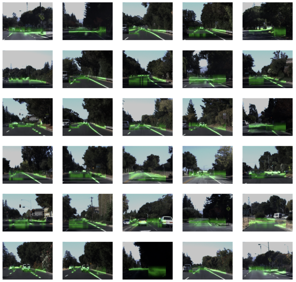
いくつかの画像については、他の車両、白線など、運転において重要な要素がハイライトされる傾向が確認できます。
これは、モデルがこれらの要素を重視して運転指示を出していることを示唆しています。
一方で、特定の方向や要素に焦点を当てず、画面の前方のピクセルを漠然とハイライトしているものも多く観察されました。
個人的には、これはモデルが特定の要素を強く参照して判断を下しているわけではなく、むしろ特に何も参照せずに直進を選択している(ステアリングを大きく切っていない)ことを示している可能性があるのかなと思いました。
まとめ
今回は自動運転車の運転判断をサポートするための深層学習モデル「PilotNet」の実装と、その判断根拠を可視化する方法について紹介しました。
Udacityのデータセットを使用して、PilotNetのトレーニングを行い、Visual Backpropagationを用いてモデルの判断根拠を可視化することができました。
可視化の結果はいまいちクリティカルにインサイトがある結果とは行かなかったですが、PilotNetの動作原理についての洞察を深めることができました。
深層学習は日々進化しており、その応用範囲も広がっています。
自動運転車の技術もその一例であり、今後もさらなる進化と発展が期待されますね。