
今年1月26日(米国時間)、Googleがオープンソース機械学習ライブラリの最新版TensorFlow 1.5を公開しました。
その時に特に注目された更新点の一つとして、TensorFlowをDefine by Runで実行できる”Eager Execution for TensorFlow”が追加されました。
TensorFlowといえばDefine and Runが特徴的ですが、その特性上デバッグなどやりづらい印象でした。
| モード | 特徴 | 代表的なライブラリ |
|---|---|---|
| Define and Run | 最初に計算グラフ(ニューラルネットワークの構造)を構築してからデータを流していく | TensorFlow |
| Define by Run | 計算グラフの構築をデータを流しながら行う | PyTorch、Chainer |
今回はTensorFlowにDefine by Runモードが追加されると聞き、実際に動かしてみて操作感を確認してみましたので、そのご共有になります。
TensorFlow Eager Executionとは?
2018年1月26日(米国時間)、Googleがオープンソース機械学習ライブラリの最新版TensorFlow 1.5を公開しました。
その時に特に注目された変更点としては、以下の機能が挙げられています。
- Eager Execution for TensorFlow
- TensorFlow Lite
- GPUアクセラレーション対応の強化
今回の本題であるEager Execution for TensorFlowは、Define by Run型のプログラミングスタイルを可能にするインタフェースで、これを有効にすると、PythonからTensorFlow演算を呼び出してすぐに実行できるようになります。
ついでに他の項目も軽く触れますと、”TensorFlow Lite”は、モバイルや組み込みデバイス向けのTensorFlowの軽量版で、学習済みのTensorFlowモデルを「.tflite」ファイルに変換しモバイルデバイスを使って低レイテンシで実行できるようになります。
“GPUアクセラレーション対応の強化”に関しては、新たにCUDA 9とcuDNN 7をサポートといったところです。
TensorFlow Eager Executionですが、GoogleはEager Execution for TensorFlowのメリットとして、下記を挙げています。
- 実行時エラーの即時確認と, Pythonツールと統合された迅速なデバッグ
- 使いやすいPython制御フローを利用した動的モデルのサポート
- カスタムおよび高次勾配の強力なサポート
- ほとんどのTensorFlow演算が利用可能
1は冒頭でも述べたように、Define and Runでは途中で値を確認するなどのデバッグをする際にもそのためのグラフをわざわざ作ってデータを流して確認しないといけませんでしたが、それが不要になり、
2については、動的に動かすことができるようになるため、if文などで計算のグラフを制御できるようになったことを意味します。
1,2がやはりDefine by Runの優位性ある特徴を大いに活用できるようになった点で分かりやすいメリットなのですが、3,4については実はよく分かっていません。
ただし今回触ってみたところ、このEagerモードでは勾配計算の部分が通常モードとだいぶ異なっているようで、これについてはあまり深掘り出来ていないのですが、便利になった点が何かしらあるのかもしれません。
4はtf.matmulなどがすぐ実行できるよってことじゃないかなと思います。
通常モードのTensorFlowでDNN
比較のため、まずは通常モードのTensorFlowの書き方を確認してみます。
問題は簡単のため、あやめの分類問題にします。
import sys, os
import numpy as np
from tqdm import tqdm
from sklearn.datasets import load_iris
from sklearn.model_selection import train_test_split
iris = load_iris()
train_x, valid_x, train_y, valid_y = train_test_split(iris.data, iris.target)
train_x.shape, train_y.shape, valid_x.shape, valid_y.shape
 # ((112, 4), (112,), (38, 4), (38,))


import tensorflow as tf

# フローの定義

input_size = 4
output_size = 3
hidden_size = 20

x_ph = tf.placeholder(tf.float32, shape=[None, input_size])
y_ph = tf.placeholder(tf.int32, [None])
y_oh = tf.one_hot(y_ph, depth=output_size, dtype=tf.float32)

fc1_w = tf.Variable(tf.truncated_normal([input_size, hidden_size], stddev=0.1), dtype=tf.float32)
fc1_b = tf.Variable(tf.constant(0.1, shape=[hidden_size]), dtype=tf.float32)
fc1 = tf.nn.relu(tf.matmul(x_ph, fc1_w) + fc1_b)

fc2_w = tf.Variable(tf.truncated_normal([hidden_size, hidden_size], stddev=0.1), dtype=tf.float32)
fc2_b = tf.Variable(tf.constant(0.1, shape=[hidden_size]), dtype=tf.float32)
fc2 = tf.nn.relu(tf.matmul(fc1, fc2_w) + fc2_b)

fc3_w = tf.Variable(tf.truncated_normal([hidden_size, output_size], stddev=0.1), dtype=tf.float32)
fc3_b = tf.Variable(tf.constant(0.1, shape=[output_size]), dtype=tf.float32)
y_pre = tf.matmul(fc2, fc3_w) + fc3_b

cross_entropy = tf.reduce_mean(tf.nn.softmax_cross_entropy_with_logits_v2(labels=y_oh, logits=y_pre))
train_step = tf.train.AdamOptimizer().minimize(cross_entropy)
correct_prediction = tf.equal(tf.argmax(y_pre, 1), tf.argmax(y_oh, 1))
accuracy = tf.reduce_mean(tf.cast(correct_prediction, tf.float32))

# 学習

epoch_num = 30
batch_size = 16

init = tf.global_variables_initializer()

with tf.Session() as sess:

    sess.run(init)

    for epoch in tqdm(range(epoch_num), file=sys.stdout):

        perm = np.random.permutation(len(train_x))

        for i in range(0, len(train_x), batch_size):

            batch_x = train_x[perm[i:i+batch_size]]
            batch_y = train_y[perm[i:i+batch_size]]
            train_step.run(feed_dict={x_ph: batch_x, y_ph: batch_y})

        train_loss = cross_entropy.eval(feed_dict={x_ph: train_x, y_ph: train_y})
        valid_loss = cross_entropy.eval(feed_dict={x_ph: valid_x, y_ph: valid_y})
        train_acc = accuracy.eval(feed_dict={x_ph: train_x, y_ph: train_y})
        valid_acc = accuracy.eval(feed_dict={x_ph: valid_x, y_ph: valid_y})

        if (epoch+1)%5 == 0:
            tqdm.write('epoch:\t{}\ttrain/loss:\t{:.5f}\tvalid/loss:\t{:.5f}\ttrain/accuracy:\t{:.5f}\tvalid/accuracy:\t{:.5f}'.format(epoch+1, train_loss, valid_loss, train_acc, valid_acc))
epoch: 5 train/loss: 1.04102 valid/loss: 1.04597 train/accuracy: 0.66964 valid/accuracy: 0.63158
epoch: 10 train/loss: 0.88552 valid/loss: 0.89669 train/accuracy: 0.67857 valid/accuracy: 0.63158
epoch: 15 train/loss: 0.63218 valid/loss: 0.64824 train/accuracy: 0.67857 valid/accuracy: 0.63158
epoch: 20 train/loss: 0.46921 valid/loss: 0.47521 train/accuracy: 0.76786 valid/accuracy: 0.71053
epoch: 25 train/loss: 0.38451 valid/loss: 0.38659 train/accuracy: 0.89286 valid/accuracy: 0.86842
epoch: 30 train/loss: 0.31372 valid/loss: 0.30514 train/accuracy: 0.97321 valid/accuracy: 1.00000
100%|██████████████████████████████| 30/30 [00:00<00:00, 115.72it/s]TensorFlowは機械学習を書く時は、低レベルAPI(生TensorFlow)の書き方と高レベルAPI(keras、layersなどを使う)の書き方があります。
使い分けとしては、
- 低レベルAPI: 機械学習や深層学習のアルゴリズムを自分で実装したい人向け
- 高レベルAPI: 機械学習や深層学習を使ってみたい人向け
に分かれると思います。
上記に記載したコードは低レベルAPIの書き方になります。
EagerモードのTensorFlowでDNN
それでは早速、Eagerモードで学習させてみます。
Eagerモードは、実行する時に下記のコマンドで初期化を行います。
import tensorflow as tf
import tensorflow.contrib.eager as tfe
tf.enable_eager_execution()

print("TensorFlow version: {}".format(tf.VERSION))
print("Eager execution: {}".format(tf.executing_eagerly()))
TensorFlow version: 1.8.0
Eager execution: Trueちなみにこれを通常モードのTensorFlowを実行した後に上記コードを実行しようとすると、
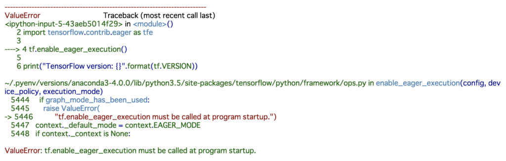
感じでエラーとなってしまいます。
どうやら実行カーネル内での通常モードとEagerモードの共存は出来ないようです。
Jupyterなどで動かしている場合はカーネルを再起動しないといけません。
逆も然りで、Eagerモードの初期化が行われた後に、通常モードのTensorFlowのコードを実行しようとすると、
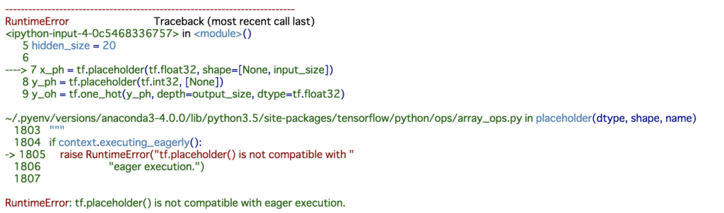
といった感じで怒られます。
同じTensorFlowなのに面白いですね。
さて、Eagerモードで学習させてみます。
実は公式のEagerモードのチュートリアルはアイリスの問題で書かれていますので、まずはサンプルコードをまるまる実行してみます。
train_dataset_url = "http://download.tensorflow.org/data/iris_training.csv"

train_dataset_fp = tf.keras.utils.get_file(fname=os.path.basename(train_dataset_url), origin=train_dataset_url)

def parse_csv(line):
    example_defaults = [[0.], [0.], [0.], [0.], [0]]  # sets field types
    parsed_line = tf.decode_csv(line, example_defaults)
    # First 4 fields are features, combine into single tensor
    features = tf.reshape(parsed_line[:-1], shape=(4,))
    # Last field is the label
    label = tf.reshape(parsed_line[-1], shape=())
    return features, label

train_dataset = tf.data.TextLineDataset(train_dataset_fp)
train_dataset = train_dataset.skip(1)             # skip the first header row
train_dataset = train_dataset.map(parse_csv)      # parse each row
train_dataset = train_dataset.shuffle(buffer_size=1000)  # randomize
train_dataset = train_dataset.batch(32)

model = tf.keras.Sequential([
    tf.keras.layers.Dense(10, activation="relu", input_shape=(4,)),  # input shape required
    tf.keras.layers.Dense(10, activation="relu"),
    tf.keras.layers.Dense(3)
])

def loss(model, x, y):
    y_ = model(x)
    return tf.losses.sparse_softmax_cross_entropy(labels=y, logits=y_)

def grad(model, inputs, targets):
    with tf.GradientTape() as tape:
        loss_value = loss(model, inputs, targets)
    return tape.gradient(loss_value, model.variables)

optimizer = tf.train.GradientDescentOptimizer(learning_rate=0.01)

train_loss_results = []
train_accuracy_results = []

num_epochs = 201

for epoch in range(num_epochs):
    epoch_loss_avg = tfe.metrics.Mean()
    epoch_accuracy = tfe.metrics.Accuracy()

    # Training loop - using batches of 32
    for x, y in train_dataset:
        # Optimize the model
        grads = grad(model, x, y)
        optimizer.apply_gradients(zip(grads, model.variables), global_step=tf.train.get_or_create_global_step())

        # Track progress
        epoch_loss_avg(loss(model, x, y))  # add current batch loss
        # compare predicted label to actual label
        epoch_accuracy(tf.argmax(model(x), axis=1, output_type=tf.int32), y)

    # end epoch
    train_loss_results.append(epoch_loss_avg.result())
    train_accuracy_results.append(epoch_accuracy.result())

    if epoch % 50 == 0:
        print("Epoch {:03d}: Loss: {:.3f}, Accuracy: {:.3%}".format(epoch, epoch_loss_avg.result(), epoch_accuracy.result()))
Epoch 000: Loss: 1.439, Accuracy: 30.000%
Epoch 050: Loss: 0.687, Accuracy: 73.333%
Epoch 100: Loss: 0.344, Accuracy: 93.333%
Epoch 150: Loss: 0.205, Accuracy: 97.500%
Epoch 200: Loss: 0.148, Accuracy: 98.333%TensorFlowの独自な関数がふんだんに使われていて、少し分かりづらいです。
少し中身を見てみますが、
train_dataset_fp = tf.keras.utils.get_file(fname=os.path.basename(train_dataset_url), origin=train_dataset_url)は直接TensorFlowからファイルポイントを取得できるようです。
これについて、
train_dataset = tf.data.TextLineDataset(train_dataset_fp)
train_dataset = train_dataset.skip(1)             # skip the first header row
train_dataset = train_dataset.map(parse_csv)      # parse each row
train_dataset = train_dataset.shuffle(buffer_size=1000)  # randomize
train_dataset = train_dataset.batch(32)
で直接CSVファイルの加工も行って、バッチサイズまで決めているようです。
Chainerのイテレータクラスあたりまでの機能を保持しているということでしょうか。
model = tf.keras.Sequential([
    tf.keras.layers.Dense(10, activation="relu", input_shape=(4,)),  # input shape required
    tf.keras.layers.Dense(10, activation="relu"),
    tf.keras.layers.Dense(3)
])

def loss(model, x, y):
    y_ = model(x)
    return tf.losses.sparse_softmax_cross_entropy(labels=y, logits=y_)

def grad(model, inputs, targets):
    with tf.GradientTape() as tape:
        loss_value = loss(model, inputs, targets)
    return tape.gradient(loss_value, model.variables)

optimizer = tf.train.GradientDescentOptimizer(learning_rate=0.01)
で、モデル、loss関数、最適化を定義しています。
モデルは高レベルAPIの書き方をしていて、loss関数は特に通常モードと変わりありませんが、勾配計算がちょっと見慣れない形になっています。
それ以降は学習となっています。
特に微分計算のところがまた特殊な形であることと、あと評価の結果を保持するためのクラスが用意されているようです。train_datasetでループすると、そのままバッチサイズごとに取り出せる模様。tf.dataは色々なファイルやデータベース等、接続先が多種多様に用意されていれば、Pythonへのデータの入力からTensorFlowの世界に閉じることができそうですね。
ともあれ、このサンプルコードだといまいち通常モードとの比較の観点でわかりづらいので、一旦、通常モードの時と同様に、scikit-learnから落としてきたデータ(numpy)からスタートするように書き直してみました。
train_x_tf = tf.convert_to_tensor(train_x, dtype=tf.float32)
train_y_tf = tf.convert_to_tensor(train_y, dtype=tf.int32)
valid_x_tf = tf.convert_to_tensor(valid_x, dtype=tf.float32)
valid_y_tf = tf.convert_to_tensor(valid_y, dtype=tf.int32)

model = tf.keras.Sequential([
    tf.keras.layers.Dense(20, activation='relu', input_shape=(4,)),
    tf.keras.layers.Dense(20, activation='relu'),
    tf.keras.layers.Dense(3)
])

def lossfun(model, x, y):
    y_pre = model(x)
    y_oh = tf.one_hot(y, depth=output_size, dtype=tf.float32)
    cross_entropy = tf.reduce_mean(tf.nn.softmax_cross_entropy_with_logits_v2(labels=y_oh, logits=y_pre))
    return cross_entropy

def grad(model, x, y):
    with tf.GradientTape() as tape:
        loss = lossfun(model, x, y)
    return tape.gradient(loss, model.variables)

epoch_num = 30
batch_size = 16

optimizer = tf.train.AdamOptimizer()

for epoch in tqdm(range(epoch_num), file=sys.stdout):

    n, _ = train_x_tf.shape
    n = n.value
    perm = np.random.permutation(n)

    for i in range(0, n, batch_size):

        batch_x = tf.gather(train_x_tf, perm[i:i+batch_size])
        batch_y = tf.gather(train_y_tf, perm[i:i+batch_size])

        grads = grad(model, batch_x, batch_y)
        optimizer.apply_gradients(zip(grads, model.variables), global_step=tf.train.get_or_create_global_step())

    train_loss = lossfun(model, train_x_tf, train_y_tf)
    correct_prediction = tf.equal(tf.argmax(model(train_x_tf), axis=1, output_type=tf.int32), train_y_tf)
    train_acc = tf.reduce_mean(tf.cast(correct_prediction, tf.float32))
    valid_loss = lossfun(model, valid_x_tf, valid_y_tf)
    correct_prediction = tf.equal(tf.argmax(model(valid_x_tf), axis=1, output_type=tf.int32), valid_y_tf)
    valid_acc = tf.reduce_mean(tf.cast(correct_prediction, tf.float32))

    if (epoch+1)%5 == 0:
        tqdm.write('epoch:\t{}\ttrain/loss:\t{:.5f}\tvalid/loss:\t{:.5f}\ttrain/accuracy:\t{:.5f}\tvalid/accuracy:\t{:.5f}'.format(
            epoch+1, train_loss, valid_loss, train_acc, valid_acc)
                  )
epoch: 5 train/loss: 0.67045 valid/loss: 0.67343 train/accuracy: 0.93750 valid/accuracy: 0.92105
epoch: 10 train/loss: 0.49943 valid/loss: 0.54966 train/accuracy: 0.77679 valid/accuracy: 0.63158
epoch: 15 train/loss: 0.41430 valid/loss: 0.46332 train/accuracy: 0.91071 valid/accuracy: 0.71053
epoch: 20 train/loss: 0.35295 valid/loss: 0.39667 train/accuracy: 0.94643 valid/accuracy: 0.89474
epoch: 25 train/loss: 0.29751 valid/loss: 0.33718 train/accuracy: 0.95536 valid/accuracy: 0.97368
epoch: 30 train/loss: 0.25024 valid/loss: 0.29310 train/accuracy: 0.97321 valid/accuracy: 0.97368
100%|██████████████████████████████| 30/30 [00:00<00:00, 30.07it/s]だいぶ理解できてきました。
train_x_tf = tf.convert_to_tensor(train_x, dtype=tf.float32)
train_y_tf = tf.convert_to_tensor(train_y, dtype=tf.int32)
valid_x_tf = tf.convert_to_tensor(valid_x, dtype=tf.float32)
valid_y_tf = tf.convert_to_tensor(valid_y, dtype=tf.int32)
確かにEagerモードとなればnumpyを触る必要もあまりありませんので、最初にnumpyをTensor型にしています。
PyTorchでいえばtorch型になると考えれば良さそうです。
モデル、微分計算は変わりありませんが、loss関数は、
def lossfun(model, x, y):
    y_pre = model(x)
    y_oh = tf.one_hot(y, depth=output_size, dtype=tf.float32)
    cross_entropy = tf.reduce_mean(tf.nn.softmax_cross_entropy_with_logits_v2(labels=y_oh, logits=y_pre))
    return cross_entropy
と、以前のようにone-hot型で評価するようにしました。
結局どちらでも良いのですが、tf.nn.softmax_cross_entropy_with_logits_v2は以前のようにラベルはone-hot型のtf.float32、tf.losses.sparse_softmax_cross_entropyはChainerなどのようにラベルをそのままtf.int32で評価できるようです。_with_logitsは、softmaxはこちらで取るので順伝播で出力されたラベル次元数のベクトルをそのまま渡してねという意味です。
学習ループに関しては、
    n, _ = train_x_tf.shape
    n = n.value
    perm = np.random.permutation(n)

    for i in range(0, n, batch_size):

        batch_x = tf.gather(train_x_tf, perm[i:i+batch_size])
        batch_y = tf.gather(train_y_tf, perm[i:i+batch_size])
でバッチを回しています。
Tensor型はnumpy型のようには扱えませんので、そのために変更しています。
numpy型だと、取得したいインデックスを配列にして複数同時にアクセスすることができますが、Tensor型ではそれをtf.gater関数で行います。
    train_loss = lossfun(model, train_x_tf, train_y_tf)
    correct_prediction = tf.equal(tf.argmax(model(train_x_tf), axis=1, output_type=tf.int32), train_y_tf)
    train_acc = tf.reduce_mean(tf.cast(correct_prediction, tf.float32))
    valid_loss = lossfun(model, valid_x_tf, valid_y_tf)
    correct_prediction = tf.equal(tf.argmax(model(valid_x_tf), axis=1, output_type=tf.int32), valid_y_tf)
valid_acc = tf.reduce_mean(tf.cast(correct_prediction, tf.float32))一旦、評価は以前と同じものにしました。metricsというクラスが用意されていることは分かりましたが、慣れてから勉強します。
と、このようにして、学習させることができましたし、なんとなく理解できてきました。
やはり通常モードと大きく違う点としては、微分計算のところがだいぶ様子が異なっています。(もしかしたらこれも同じように書き直せるのかもしれないですが)
どうやらGradientTapeクラスが、dloss/dwの微分計算を担当するようで、tape = tfe.GradientTape()としてtape(loss, w)とするようです。
ここは慣れは必要ですね。
また、上記は高レベルAPIの書き方なので、以下はちょっと生TensorFlowの低レベルAPIの書き方に寄せてみた例です。
"""
model = tf.keras.Sequential([
    tf.keras.layers.Dense(20, activation='relu', input_shape=(4,)),
    tf.keras.layers.Dense(20, activation='relu'),
    tf.keras.layers.Dense(3)
])
"""
class Model():

    def __init__(self):
        input_size = 4
        output_size = 3
        hidden_size = 20
        self.fc1_w = tfe.Variable(tf.truncated_normal([input_size, hidden_size], stddev=0.1), dtype=tf.float32)
        self.fc1_b = tfe.Variable(tf.constant(0.1, shape=[hidden_size]), dtype=tf.float32)
        self.fc2_w = tfe.Variable(tf.truncated_normal([hidden_size, hidden_size], stddev=0.1), dtype=tf.float32)
        self.fc2_b = tfe.Variable(tf.constant(0.1, shape=[hidden_size]), dtype=tf.float32)
        self.fc3_w = tfe.Variable(tf.truncated_normal([hidden_size, output_size], stddev=0.1), dtype=tf.float32)
        self.fc3_b = tfe.Variable(tf.constant(0.1, shape=[output_size]), dtype=tf.float32)
        self.variables = [
            self.fc1_w, self.fc1_b,
            self.fc2_w, self.fc2_b,
            self.fc3_w, self.fc3_b
        ]

    def __call__(self, x):
        h = tf.nn.relu(tf.matmul(x, self.fc1_w) + self.fc1_b)
        h = tf.nn.relu(tf.matmul(h, self.fc2_w) + self.fc2_b)
        y_pre = tf.matmul(h, self.fc3_w) + self.fc3_b
        return y_pre

model = Model()

def lossfun(model, x, y):
    y_pre = model(x)
    y_oh = tf.one_hot(y, depth=output_size, dtype=tf.float32)
    cross_entropy = tf.reduce_mean(tf.nn.softmax_cross_entropy_with_logits_v2(labels=y_oh, logits=y_pre))
    return cross_entropy

def grad(model, x, y):
    with tf.GradientTape() as tape:
        loss = lossfun(model, x, y)
    return tape.gradient(loss, model.variables)

train_x_tf = tf.convert_to_tensor(train_x, dtype=tf.float32)
train_y_tf = tf.convert_to_tensor(train_y, dtype=tf.int32)
valid_x_tf = tf.convert_to_tensor(valid_x, dtype=tf.float32)
valid_y_tf = tf.convert_to_tensor(valid_y, dtype=tf.int32)

epoch_num = 30
batch_size = 16

optimizer = tf.train.AdamOptimizer()

for epoch in tqdm(range(epoch_num), file=sys.stdout):

    n, _ = train_x_tf.shape
    n = n.value
    perm = np.random.permutation(n)

    for i in range(0, n, batch_size):

        batch_x = tf.gather(train_x_tf, perm[i:i+batch_size])
        batch_y = tf.gather(train_y_tf, perm[i:i+batch_size])

        grads = grad(model, batch_x, batch_y)
        optimizer.apply_gradients(zip(grads, model.variables), global_step=tf.train.get_or_create_global_step())

    train_loss = lossfun(model, train_x_tf, train_y_tf)
    correct_prediction = tf.equal(tf.argmax(model(train_x_tf), axis=1, output_type=tf.int32), train_y_tf)
    train_acc = tf.reduce_mean(tf.cast(correct_prediction, tf.float32))
    valid_loss = lossfun(model, valid_x_tf, valid_y_tf)
    correct_prediction = tf.equal(tf.argmax(model(valid_x_tf), axis=1, output_type=tf.int32), valid_y_tf)
    valid_acc = tf.reduce_mean(tf.cast(correct_prediction, tf.float32))

    if (epoch+1)%5 == 0:
        tqdm.write('epoch:\t{}\ttrain/loss:\t{:.5f}\tvalid/loss:\t{:.5f}\ttrain/accuracy:\t{:.5f}\tvalid/accuracy:\t{:.5f}'.format(
            epoch+1, train_loss, valid_loss, train_acc, valid_acc)
                  )
epoch: 5 train/loss: 0.97063 valid/loss: 0.97965 train/accuracy: 0.74107 valid/accuracy: 0.60526
epoch: 10 train/loss: 0.74250 valid/loss: 0.78540 train/accuracy: 0.69643 valid/accuracy: 0.57895
epoch: 15 train/loss: 0.52186 valid/loss: 0.58941 train/accuracy: 0.69643 valid/accuracy: 0.57895
epoch: 20 train/loss: 0.40647 valid/loss: 0.46311 train/accuracy: 0.83929 valid/accuracy: 0.68421
epoch: 25 train/loss: 0.33188 valid/loss: 0.38010 train/accuracy: 0.93750 valid/accuracy: 0.84211
epoch: 30 train/loss: 0.26992 valid/loss: 0.30254 train/accuracy: 0.96429 valid/accuracy: 0.97368
100%|██████████████████████████████| 30/30 [00:00<00:00, 32.57it/s]変数はtf.Variableではなくtfe.Variableを使います。
これで自分で変数までも定義させた上で、Eagerモードで実行することができました。
ちなみに、先ほどの高レベルAPIの書き方はkerasを使いましたが、kerasじゃない書き方(tf.layers)をする場合は下記のようにtfe.Networkクラスを使うのが便利そうです。
class Model(tfe.Network):

    def __init__(self):
        super(Model, self).__init__()
        input_size = 4
        output_size = 3
        hidden_size = 20
        self.fc1 = self.track_layer(tf.layers.Dense(hidden_size, input_shape=(input_size, )))
        self.fc2 = self.track_layer(tf.layers.Dense(hidden_size, input_shape=(hidden_size, )))
        self.fc3 = self.track_layer(tf.layers.Dense(output_size, input_shape=(hidden_size, )))

    def __call__(self, x):
        h = tf.nn.relu(self.fc1(x))
        h = tf.nn.relu(self.fc2(h))
        y = self.fc3(h)
        return y

model = Model()

def lossfun(model, x, y):
    y_pre = model(x)
    y_oh = tf.one_hot(y, depth=output_size, dtype=tf.float32)
    cross_entropy = tf.reduce_mean(tf.nn.softmax_cross_entropy_with_logits_v2(labels=y_oh, logits=y_pre))
    return cross_entropy

def grad(model, x, y):
    with tf.GradientTape() as tape:
        loss = lossfun(model, x, y)
    return tape.gradient(loss, model.variables)

train_x_tf = tf.convert_to_tensor(train_x, dtype=tf.float32)
train_y_tf = tf.convert_to_tensor(train_y, dtype=tf.int32)
valid_x_tf = tf.convert_to_tensor(valid_x, dtype=tf.float32)
valid_y_tf = tf.convert_to_tensor(valid_y, dtype=tf.int32)

epoch_num = 30
batch_size = 16

optimizer = tf.train.AdamOptimizer()

for epoch in tqdm(range(epoch_num), file=sys.stdout):

    n, _ = train_x_tf.shape
    n = n.value
    perm = np.random.permutation(n)

    for i in range(0, n, batch_size):

        batch_x = tf.gather(train_x_tf, perm[i:i+batch_size])
        batch_y = tf.gather(train_y_tf, perm[i:i+batch_size])

        grads = grad(model, batch_x, batch_y)
        optimizer.apply_gradients(zip(grads, model.variables), global_step=tf.train.get_or_create_global_step())

    train_loss = lossfun(model, train_x_tf, train_y_tf)
    correct_prediction = tf.equal(tf.argmax(model(train_x_tf), axis=1, output_type=tf.int32), train_y_tf)
    train_acc = tf.reduce_mean(tf.cast(correct_prediction, tf.float32))
    valid_loss = lossfun(model, valid_x_tf, valid_y_tf)
    correct_prediction = tf.equal(tf.argmax(model(valid_x_tf), axis=1, output_type=tf.int32), valid_y_tf)
    valid_acc = tf.reduce_mean(tf.cast(correct_prediction, tf.float32))

    if (epoch+1)%5 == 0:
        tqdm.write('epoch:\t{}\ttrain/loss:\t{:.5f}\tvalid/loss:\t{:.5f}\ttrain/accuracy:\t{:.5f}\tvalid/accuracy:\t{:.5f}'.format(
            epoch+1, train_loss, valid_loss, train_acc, valid_acc)
                  )
epoch: 5 train/loss: 0.93403 valid/loss: 0.91708 train/accuracy: 0.60714 valid/accuracy: 0.73684
epoch: 10 train/loss: 0.75861 valid/loss: 0.77444 train/accuracy: 0.72321 valid/accuracy: 0.60526
epoch: 15 train/loss: 0.62497 valid/loss: 0.65579 train/accuracy: 0.70536 valid/accuracy: 0.57895
epoch: 20 train/loss: 0.52212 valid/loss: 0.55455 train/accuracy: 0.83036 valid/accuracy: 0.65789
epoch: 25 train/loss: 0.42839 valid/loss: 0.46885 train/accuracy: 0.87500 valid/accuracy: 0.73684
epoch: 30 train/loss: 0.37426 valid/loss: 0.40928 train/accuracy: 0.91964 valid/accuracy: 0.86842
100%|██████████████████████████████| 30/30 [00:01 <00:00, 23.05it/s]このように高レベルAPIの使い方+Eagerで書いていると、やはりChainerやPyTorchになんとなくコードの構成が似てきます。
これでEagerモードの使い方が分かりましたし、動的なグラフをTensorFlowで学習させることができるようになりました。
例えば、何の意味もないですが、以下のように無駄にもう一つ順伝播を通ったり通らなかったりみたいなネットワークも、Pythonのif文で学習させることができます。
class Model(tfe.Network):

    def __init__(self):
        super(Model, self).__init__()
        input_size = 4
        output_size = 3
        hidden_size = 20
        self.fc1 = self.track_layer(tf.layers.Dense(hidden_size, input_shape=(input_size, )))
        self.fc2 = self.track_layer(tf.layers.Dense(hidden_size, input_shape=(hidden_size, )))

        self.fc2_2 = self.track_layer(tf.layers.Dense(hidden_size, input_shape=(hidden_size, ))) # もう一つ無駄に順伝播作って

        self.fc3 = self.track_layer(tf.layers.Dense(output_size, input_shape=(hidden_size, )))

    def __call__(self, x):

        h = tf.nn.relu(self.fc1(x))
        h = tf.nn.relu(self.fc2(h))

        # ランダムにもう一つ無駄に通すという意味のない分岐をするネットワーク
        prob = np.random.randn()
        if prob > 0:
            h = tf.nn.relu(self.fc2_2(h))

        y = self.fc3(h)
        return y

model = Model()

def lossfun(model, x, y):
    y_pre = model(x)
    y_oh = tf.one_hot(y, depth=output_size, dtype=tf.float32)
    cross_entropy = tf.reduce_mean(tf.nn.softmax_cross_entropy_with_logits_v2(labels=y_oh, logits=y_pre))
    return cross_entropy

def grad(model, x, y):
    with tf.GradientTape() as tape:
        loss = lossfun(model, x, y)
    return tape.gradient(loss, model.variables)

train_x_tf = tf.convert_to_tensor(train_x, dtype=tf.float32)
train_y_tf = tf.convert_to_tensor(train_y, dtype=tf.int32)
valid_x_tf = tf.convert_to_tensor(valid_x, dtype=tf.float32)
valid_y_tf = tf.convert_to_tensor(valid_y, dtype=tf.int32)

epoch_num = 30
batch_size = 16

optimizer = tf.train.AdamOptimizer()

for epoch in tqdm(range(epoch_num), file=sys.stdout):

    n, _ = train_x_tf.shape
    n = n.value
    perm = np.random.permutation(n)

    for i in range(0, n, batch_size):

        batch_x = tf.gather(train_x_tf, perm[i:i+batch_size])
        batch_y = tf.gather(train_y_tf, perm[i:i+batch_size])

        grads = grad(model, batch_x, batch_y)
        optimizer.apply_gradients(zip(grads, model.variables), global_step=tf.train.get_or_create_global_step())

    train_loss = lossfun(model, train_x_tf, train_y_tf)
    correct_prediction = tf.equal(tf.argmax(model(train_x_tf), axis=1, output_type=tf.int32), train_y_tf)
    train_acc = tf.reduce_mean(tf.cast(correct_prediction, tf.float32))
    valid_loss = lossfun(model, valid_x_tf, valid_y_tf)
    correct_prediction = tf.equal(tf.argmax(model(valid_x_tf), axis=1, output_type=tf.int32), valid_y_tf)
    valid_acc = tf.reduce_mean(tf.cast(correct_prediction, tf.float32))

    if (epoch+1)%5 == 0:
        tqdm.write('epoch:\t{}\ttrain/loss:\t{:.5f}\tvalid/loss:\t{:.5f}\ttrain/accuracy:\t{:.5f}\tvalid/accuracy:\t{:.5f}'.format(
            epoch+1, train_loss, valid_loss, train_acc, valid_acc)
                  )
epoch: 5 train/loss: 1.01586 valid/loss: 1.03447 train/accuracy: 0.36607 valid/accuracy: 0.23684
epoch: 10 train/loss: 0.80235 valid/loss: 0.76231 train/accuracy: 0.64286 valid/accuracy: 0.76316
epoch: 15 train/loss: 0.73061 valid/loss: 0.69120 train/accuracy: 0.77679 valid/accuracy: 0.57895
epoch: 20 train/loss: 0.58115 valid/loss: 0.61735 train/accuracy: 0.69643 valid/accuracy: 0.57895
epoch: 25 train/loss: 0.56904 valid/loss: 0.52894 train/accuracy: 0.93750 valid/accuracy: 0.57895
epoch: 30 train/loss: 0.50970 valid/loss: 0.48441 train/accuracy: 0.70536 valid/accuracy: 0.89474
100%|██████████████████████████████| 30/30 [00:00<00:00, 30.55it/s]
値があっちにいったりこっちにいったりするネットワークなので、当然学習が安定しません。
面白い。
この程度なら別にプレースホルダーに確率値を供給することで通常モードでも可能ですが、データによってとか、バッチごとに異なるネットワークを通したい時には使えるということになりそうです。
EagerモードのTensorFlowでCNN
さらにおまけですが、EagerモードでCNN(畳み込みニューラルネットワーク)の学習もさせてみましたので、コード例をご共有して終わりにしようと思います。
from sklearn.datasets import fetch_mldata

mnist = fetch_mldata('MNIST original')
mnist['data'] = mnist['data'].astype(np.float32).reshape(len(mnist['data']), 28, 28, 1) # image data
mnist['data'] /= 255
mnist['target'] = mnist['target'].astype(np.int32) # label data
mnist['data'].shape, mnist['target'].shape # ((70000, 28, 28, 1), (70000,))

# train data size : validation data size= 8 : 2
train_x, valid_x, train_y, valid_y = model_selection.train_test_split(mnist['data'], mnist['target'], test_size=0.2)
train_x.shape, train_y.shape, valid_x.shape, valid_y.shape # ((56000, 28, 28, 1), (56000,), (14000, 28, 28, 1), (14000,))

epoch_num = 5
batch_size = 1000
output_size = 10

model = tf.keras.models.Sequential([
    tf.keras.layers.Conv2D(20, (5, 5), activation=tf.nn.relu),
    tf.keras.layers.Conv2D(50, (5, 5), activation=tf.nn.relu),
    tf.keras.layers.Flatten(),
    tf.keras.layers.Dense(500, activation=tf.nn.relu),
    tf.keras.layers.Dense(500, activation=tf.nn.relu),
    tf.keras.layers.Dense(output_size, activation=tf.nn.softmax),
])

def lossfun(model, x, y):
    y_pre = model(x)
    y_oh = tf.one_hot(y, depth=output_size, dtype=tf.float32)
    cross_entropy = tf.reduce_mean(tf.nn.softmax_cross_entropy_with_logits_v2(labels=y_oh, logits=y_pre))
    return cross_entropy

def grad(model, x, y):
    with tf.GradientTape() as tape:
        loss = lossfun(model, x, y)
    return tape.gradient(loss, model.variables)

optimizer = tf.train.AdamOptimizer()

train_x_tf = tf.convert_to_tensor(train_x, dtype=tf.float32)
train_y_tf = tf.convert_to_tensor(train_y, dtype=tf.int32)
valid_x_tf = tf.convert_to_tensor(valid_x, dtype=tf.float32)
valid_y_tf = tf.convert_to_tensor(valid_y, dtype=tf.int32)

for epoch in tqdm(range(epoch_num), file=sys.stdout):

    n = train_x_tf.shape[0]
    n = n.value
    perm = np.random.permutation(n)

    for i in range(0, n, batch_size):

        batch_x = tf.gather(train_x_tf, perm[i:i+batch_size])
        batch_y = tf.gather(train_y_tf, perm[i:i+batch_size])

        grads = grad(model, batch_x, batch_y)
        optimizer.apply_gradients(zip(grads, model.variables), global_step=tf.train.get_or_create_global_step())

    train_loss = lossfun(model, train_x_tf, train_y_tf)
    correct_prediction = tf.equal(tf.argmax(model(train_x_tf), axis=1, output_type=tf.int32), train_y_tf)
    train_acc = tf.reduce_mean(tf.cast(correct_prediction, tf.float32))
    valid_loss = lossfun(model, valid_x_tf, valid_y_tf)
    correct_prediction = tf.equal(tf.argmax(model(valid_x_tf), axis=1, output_type=tf.int32), valid_y_tf)
    valid_acc = tf.reduce_mean(tf.cast(correct_prediction, tf.float32))

    if (epoch+1)%1 == 0:
        tqdm.write('epoch:\t{}\ttrain/loss:\t{:.5f}\tvalid/loss:\t{:.5f}\ttrain/accuracy:\t{:.5f}\tvalid/accuracy:\t{:.5f}'.format(
            epoch+1, train_loss, valid_loss, train_acc, valid_acc)
        )
epoch: 1 train/loss: 1.53761 valid/loss: 1.53892 train/accuracy: 0.92557 valid/accuracy: 0.92314
epoch: 2 train/loss: 1.48837 valid/loss: 1.49182 train/accuracy: 0.97371 valid/accuracy: 0.97029
epoch: 3 train/loss: 1.48066 valid/loss: 1.48491 train/accuracy: 0.98150 valid/accuracy: 0.97693
epoch: 4 train/loss: 1.47476 valid/loss: 1.47896 train/accuracy: 0.98702 valid/accuracy: 0.98314
epoch: 5 train/loss: 1.47420 valid/loss: 1.47815 train/accuracy: 0.98782 valid/accuracy: 0.98336
100%|██████████| 5/5 [00:16<00:00, 3.36s/it]preds = np.argmax(model.predict(valid_x), axis=1)
cm = metrics.confusion_matrix(preds, valid_y)
plt.figure(figsize=(10,8))
sns.heatmap(cm, annot=True, fmt='d')
plt.show()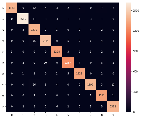
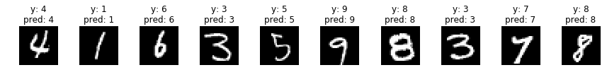
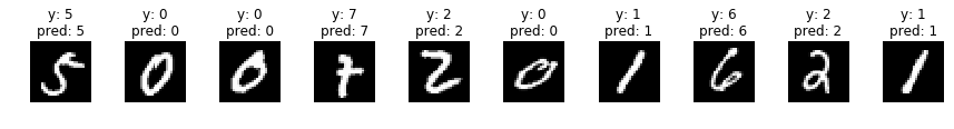
indices = np.random.choice(len(valid_x), 30)

for i, idx in enumerate(indices):

    if i%10 == 0:
        fig, axs = plt.subplots(ncols=10, figsize=(15,1))

    x = valid_x[idx]
    y = valid_y[idx]

    x_img = x.reshape(28, 28)
    x = x[np.newaxis]

    p = np.argmax(model.predict(x), axis=1)[0]

    axs[i%10].imshow(x_img, cmap='gray')
    title = 'y: {}'.format(y) + '\n' + 'pred: {}'.format(p)
    axs[i%10].set_title(title)
    axs[i%10].axis('off')

plt.show()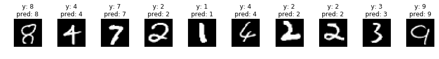
まとめ
今回はTensorFlowに追加されたDefine by Run機能Eager Executionについて、基本的な操作方法をご紹介しました。
やはりこのモードは、これまでのTensorFlow通常モードと比較すると、より直感的なモデルの構築とデバッグを大幅に容易にしてくれます。
一方で、あえて欠点に関して挙げるならば、計算グラフ最適化ができないためにパフォーマンスが低下する場合があることが挙げられると思います。
そのような場合は作成したネットワークを元に通常モードで組み直して切り替えることもできることを覚えておいた方が良いでしょう。
是非、Eager Executionを活用して、自身の機械学習プロジェクトをより効率的に進めてみてください。