自動運転向け深層学習モデルの判断根拠を解析してみる｜コラム

※本コラムは、以前に個人ブログとして公開していた内容を、加筆・再構成のうえ掲載しております。技術的な内容は執筆当時のものであり、現在とは異なる場合がございます。

こんにちは。Anagraftの伊藤です。

今回は、NVIDIAが公開した自動運転向け深層学習モデルの実験記事にインスパイアされた取り組みをご紹介します。車載カメラの画像から直接ステアリング操作を出力する「PilotNet」というモデルを実装し、そのモデルが画像のどこを見て運転判断をしているのか、判断根拠を可視化してみます。

元記事の執筆は2018年で、当時はEnd-to-End方式の自動運転がまだ研究段階の話題でしたが、その後この方式は実用化の主役になりつつあります。記事の後半では、その最新動向にも触れます。

著者伊藤瑛志

Anagraft（アナグラフト）合同会社代表 AXプロジェクト顧問・支援
データサイエンティスト since 2013 BCG／ALBERT（現アクセンチュア）出身

NVIDIAの実験にインスパイアされて
データセットの準備
PilotNetについて
Visual Backpropagationによるステアリング操作要因の可視化
まとめ
その後の発展・最新動向（2026年時点）
参考文献

NVIDIAの実験にインスパイアされて

今回は、以下のNVIDIAの記事にインスパイアされた取り組みになります。

Explaining How End-to-End Deep Learning Steers a Self-Driving Car（NVIDIA Technical Blog）

上記の記事では、NVIDIAが提案した深層学習モデルPilotNetを使った実験が紹介されています。 PilotNetは、自動運転車の運転判断をサポートするための深層学習モデルです。車載カメラの画像を入力し、それに基づいてEnd-to-Endで運転操作（例えば、ステアリング操作）を出力するモデルです。

さらに記事では、そのようにして学習されたPilotNetが、運転操作を出力するために画像のどの部分を注視しているのかといった判断根拠を可視化する試みも行っています。

今回は、自動運転向けに収集・公開されたデータセットを使って同様の実験を試してみます。

データセットの準備

PilotNetを実装する上で、まずは自動運転のための画像とステアリング操作のデータセットを準備します。今回の実装では、以下のUdacityが提供する自動運転車のデータセットを使用します。データセットには、実際の道路環境での運転時の画像とセンサーデータが記録されており、学習に適していそうです。

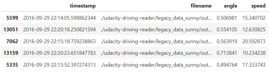
https://github.com/rwightman/udacity-driving-reader

実際にデータの中身を確認してみて、今回使うカラムに限定すると以下のようなデータセットになっています。（なお、以降のコードは要点を抜き出した抜粋であり、import文やデータ準備の一部は紙面の都合上省略しています。）

import functools
import numpy as np
import pandas as pd
import matplotlib
import matplotlib.pyplot as plt
from PIL import Image

target_output_path = './udacity-driving-reader/legacy_data_sunny/output/'

df_camera = pd.read_csv(target_output_path + 'camera.csv')
df_steering = pd.read_csv(target_output_path + 'steering.csv')

df_camera = df_camera[df_camera['frame_id'] == 'center_camera']
df_camera['timestamp'] = pd.to_datetime(df_camera['timestamp'])
df_camera.set_index(['timestamp'], inplace=True)
df_camera.index.rename('index', inplace=True)

df_steering['timestamp'] = pd.to_datetime(df_steering['timestamp'])
df_steering.set_index(['timestamp'], inplace=True)
df_steering.index.rename('index', inplace=True)

df_merged = functools.reduce(lambda left, right: pd.merge(left, right, how='outer', left_index=True, right_index=True), [df_camera, df_steering])
df_merged.interpolate(method='time', inplace=True)
df_filtered = df_merged.loc[df_camera.index]
df_filtered.fillna(0.0, inplace=True)
df_filtered.index.rename('timestamp', inplace=True)
df_filtered = df_filtered.reset_index()
df_filtered = df_filtered[['timestamp', 'filename', 'angle', 'speed']]
df_filtered['filename'] = target_output_path + df_filtered['filename']

# 停止している画像・不自然にハンドルが切れすぎている画像を除き、正規化
df_filtered = df_filtered[10 < df_filtered['speed']]
df_filtered = df_filtered[(-0.5 <= df_filtered['angle']) & (df_filtered['angle'] <= 0.5)]
df_filtered['angle'] += 0.5
df_filtered = df_filtered.sample(frac=1)

df_filtered.head()

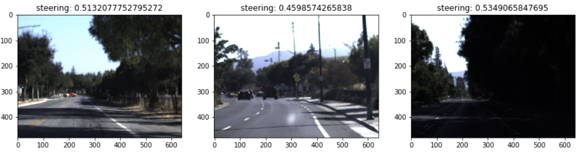
データセットには画像パスが格納されていますので、何枚か画像を表示してみると以下のような感じです。

df = df_filtered.sample(frac=1)[:3]

fig, axs = plt.subplots(ncols=3, figsize=(15, 4))

for i, (index, row) in enumerate(df.iterrows()):
    img = Image.open(row['filename'])
    axs[i].imshow(img)
    axs[i].set_title('steering: {}'.format(row['angle']))

plt.show()

PilotNetについて

冒頭で述べました通り、PilotNetは、NVIDIAが提案するディープラーニングモデルで、自動運転車の運転判断をサポートするために設計されました。このモデルは、カメラからの入力画像を受け取り、それに基づいて運転指示（例: ハンドルの角度）を出力します。論文は以下です。

Bojarski, M., et al. (2017). Explaining How a Deep Neural Network Trained with End-to-End Learning Steers a Car. arXiv:1704.07911

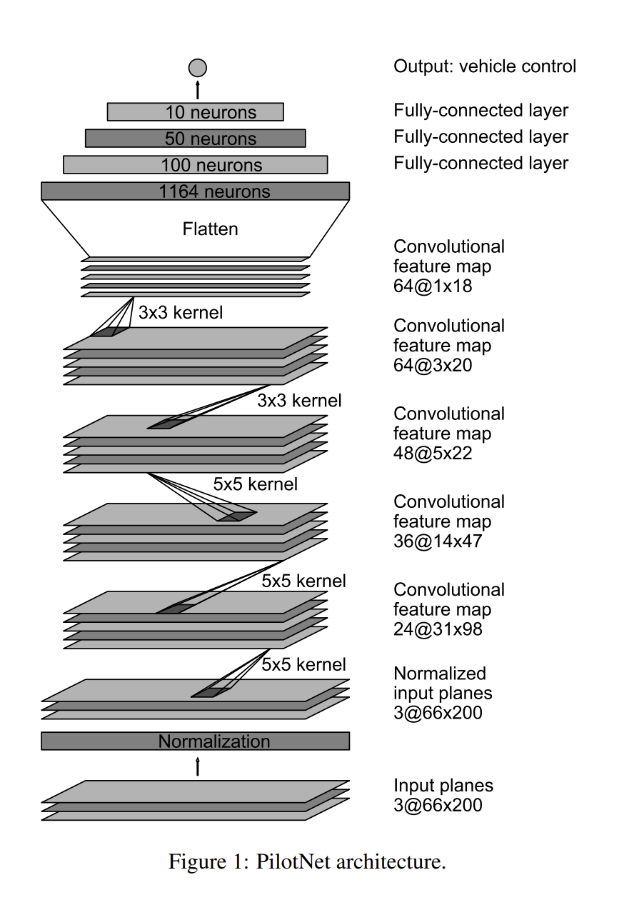
PilotNetのアーキテクチャは、畳み込みニューラルネットワーク（CNN）をベースにしています。このネットワークは、複数の畳み込み層、活性化関数、および全結合層から構成されています。以下は論文から抜粋のアーキテクチャ図です。

モデルの実装は以下の通りです。元記事では深層学習ライブラリにChainerを使用していました。Chainerは2019年末に開発が終了しPyTorchへ開発リソースが移管されたため、現在から新規に取り組む場合はPyTorchやTensorFlowでの実装をおすすめしますが、ここでは元記事の記録として当時のChainer実装を残します（移植の考え方は後述します）。

class PilotNet(chainer.Chain):

    def __init__(self):
        super(PilotNet, self).__init__()
        with self.init_scope():
            self.bn0 = L.BatchNormalization(3)
            self.conv1 = L.Convolution2D(3, 24, ksize=5, stride=2)
            self.conv2 = L.Convolution2D(24, 36, ksize=5, stride=2)
            self.conv3 = L.Convolution2D(36, 48, ksize=5, stride=2)
            self.conv4 = L.Convolution2D(48, 64, ksize=3)
            self.conv5 = L.Convolution2D(64, 64, ksize=3)
            self.fc6 = L.Linear(None, 100)
            self.fc7 = L.Linear(100, 50)
            self.fc8 = L.Linear(50, 10)
            self.fc9 = L.Linear(10, 1)

    def __call__(self, x, extract_feature=False):
        h0 = self.bn0(x)
        h1 = F.relu(self.conv1(h0))
        h2 = F.relu(self.conv2(h1))
        h3 = F.relu(self.conv3(h2))
        h4 = F.relu(self.conv4(h3))
        h5 = F.relu(self.conv5(h4))
        h6 = F.dropout(F.relu(self.fc6(h5)), ratio=0.1)
        h7 = F.dropout(F.relu(self.fc7(h6)), ratio=0.1)
        h8 = F.dropout(F.relu(self.fc8(h7)), ratio=0.1)
        y = self.fc9(h8)

        if extract_feature:
            return {'conv1': h1, 'conv2': h2, 'conv3': h3, 'conv4': h4, 'conv5': h5, 'fc6': h6, 'fc7': h7, 'fc8': h8, 'fc9': y}

        return y

    def get_mask(self, x):
        h0 = self.bn0(x)
        h1 = F.relu(self.conv1(h0))
        h2 = F.relu(self.conv2(h1))
        h3 = F.relu(self.conv3(h2))
        h4 = F.relu(self.conv4(h3))
        h5 = F.relu(self.conv5(h4))

        h5 = F.mean(h5, axis=1)
        h5 = F.reshape(h5, (h5.data.shape[0], 1, h5.data.shape[1], h5.data.shape[2]))
        h5 = chainer.cuda.to_cpu(h5.data)
        h4_rev = L.Deconvolution2D(1, 1, ksize=3,
                                 initialW=np.ones((1, 1, 3, 3), dtype=np.float32),
                                 initial_bias=np.zeros((1), dtype=np.float32))(h5)
        h4 = F.mean(h4, axis=1)
        h4 = F.reshape(h4, (h4.data.shape[0], 1, h4.data.shape[1], h4.data.shape[2]))
        h4 = chainer.cuda.to_cpu(h4.data)
        h3_rev = L.Deconvolution2D(1, 1, ksize=3,
                                  initialW=np.ones((1, 1, 3, 3), dtype=np.float32),
                                  initial_bias=np.zeros((1), dtype=np.float32))(h4_rev*h4)
        h3 = F.mean(h3, axis=1)
        h3 = F.reshape(h3, (h3.data.shape[0], 1, h3.data.shape[1], h3.data.shape[2]))
        h3 = chainer.cuda.to_cpu(h3.data)
        h2_rev = L.Deconvolution2D(1, 1, ksize=5, stride=2, outsize=(h2.data.shape[2], h2.data.shape[3]),
                                  initialW=np.ones((1, 1, 5, 5), dtype=np.float32),
                                  initial_bias=np.zeros((1), dtype=np.float32))(h3_rev*h3)
        h2 = F.mean(h2, axis=1)
        h2 = F.reshape(h2, (h2.data.shape[0], 1, h2.data.shape[1], h2.data.shape[2]))
        h2 = chainer.cuda.to_cpu(h2.data)
        h1_rev = L.Deconvolution2D(1, 1, ksize=5, stride=2, outsize=(h1.data.shape[2], h1.data.shape[3]),
                                  initialW=np.ones((1, 1, 5, 5), dtype=np.float32),
                                  initial_bias=np.zeros((1), dtype=np.float32))(h2_rev*h2)
        h1 = F.mean(h1, axis=1)
        h1 = F.reshape(h1, (h1.data.shape[0], 1, h1.data.shape[1], h1.data.shape[2]))
        h1 = chainer.cuda.to_cpu(h1.data)
        mask = L.Deconvolution2D(1, 1, ksize=5, stride=2, outsize=(h0.data.shape[2], h0.data.shape[3]),
                                initialW=np.ones((1, 1, 5, 5), dtype=np.float32),
                                initial_bias=np.zeros((1), dtype=np.float32))(h1_rev*h1)

        return mask

モデルのトレーニングには、先ほどの「データセットの準備」で取得したUdacityのデータセットを使用します。したがって、入力は車載画像で出力値はステアリング（ハンドル）の角度です。学習のコードは以下の通りです。

model = L.Classifier(PilotNet(), lossfun=F.mean_squared_error)
model.compute_accuracy = False
optimizer = chainer.optimizers.Adam(alpha=1e-4)
optimizer.setup(model)

if gpu >= 0:
    chainer.cuda.get_device(gpu).use()
    model.to_gpu(gpu)

epoch_num = 100
batch_size = 1000

train_iter = chainer.iterators.SerialIterator(train_dataset, batch_size)
test_iter = chainer.iterators.SerialIterator(valid_dataset, batch_size, repeat=False, shuffle=False)
updater = chainer.training.StandardUpdater(train_iter, optimizer, device=gpu)
trainer = chainer.training.Trainer(updater, (epoch_num, 'epoch'), out='result_pilotnet')
trainer.extend(extensions.Evaluator(test_iter, model, device=gpu))
trainer.extend(extensions.LogReport(trigger=(10, 'epoch')))
trainer.extend(extensions.LogReport())
trainer.extend(extensions.PrintReport(['epoch', 'main/loss', 'validation/main/loss', 'elapsed_time']))
trainer.extend(extensions.PlotReport(['main/loss', 'validation/main/loss'], 'epoch', file_name='loss.png'))
trainer.extend(extensions.snapshot(filename='snapshot_epoch_{.updater.epoch}.npz'), trigger=(epoch_num, 'epoch'))
trainer.run()

epoch       main/loss   validation/main/loss  elapsed_time
10          0.0309514   0.0388316             82.0616
20          0.0122537   0.00430815            149.306
30          0.00964154  0.00319876            216.603
40          0.0084587   0.00268209            284.642
50          0.00782145  0.0022793             351.935
60          0.00739421  0.00230404            419.19
70          0.00697377  0.00171783            487.325
80          0.00672234  0.00163945            554.637
90          0.00637599  0.00138362            622.032
100         0.00623202  0.00120607            690.019

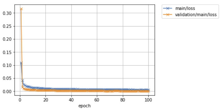
問題なく学習させることができました。

Visual Backpropagationによるステアリング操作要因の可視化

NVIDIAの記事では、PilotNetの判断を明確に理解するための方法として、VisualBackPropと呼ばれる可視化手法を試しています。名前に「Backprop」とありますが、これは通常の勾配の逆伝播そのものではなく、各畳み込み層の特徴マップをチャンネル方向に平均し、それを逆畳み込みによって入力側へ一段ずつ投影していくことで、モデルの判断に寄与した領域を浮かび上がらせる手法です。これにより、入力画像のどの部分がモデルの判断に大きく寄与しているのかを特定することができます。

実際にやってみると以下のようになりました。

from sklearn.preprocessing import MinMaxScaler
from PIL import ImageEnhance

col_num = 5
for i, (x, y) in enumerate(zip(valid_x, valid_y)):

    if i >= 30:
        break
    if i % col_num == 0:
        fig, axs = plt.subplots(ncols=col_num, figsize=(20, 4))

    img = Image.open(x)

    x = processing_x(img)
    x = x[np.newaxis]

    mask = model.predictor.get_mask(x)
    mask = MinMaxScaler().fit_transform(mask.data.squeeze())

    w, h = img.size
    mask *= 255
    mask = Image.fromarray(mask).convert('L')
    mask = mask.resize((((w//8)*7 - (w//8)*1), ((h//8)*8 - (h//8)*5)))
    mask = Image.merge('RGB', (mask.point(lambda x: x * 0 / 255), mask.point(lambda x: x * 255 / 255), mask.point(lambda x: x * 0 / 255)))

    overlay = Image.new('RGB', (w, h))
    overlay.paste(mask, ((w//8)*1, (h//8)*5))

    blended = Image.blend(img, overlay, 0.4)
    enhancer = ImageEnhance.Brightness(blended)
    blended = enhancer.enhance(1.3)
    axs[i % col_num].imshow(blended)
    axs[i % col_num].axis('off')

plt.show()

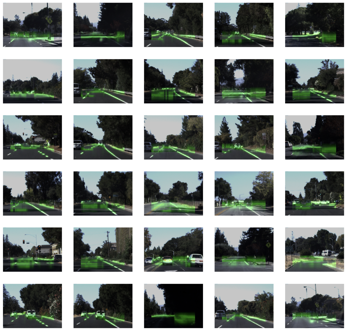
いくつかの画像については、他の車両、白線など、運転において重要な要素がハイライトされる傾向が確認できます。これは、モデルがこれらの要素を重視して運転指示を出していることを示唆しています。

一方で、特定の方向や要素に焦点を当てず、画面の前方のピクセルを漠然とハイライトしているものも多く観察されました。個人的には、これはモデルが特定の要素を強く参照して判断を下しているわけではなく、むしろ特に何も参照せずに直進を選択している（ステアリングを大きく切っていない）ことを示している可能性があるのかなと思いました。

まとめ

今回は自動運転車の運転判断をサポートするための深層学習モデル「PilotNet」の実装と、その判断根拠を可視化する方法について紹介しました。 Udacityのデータセットを使用して、PilotNetのトレーニングを行い、Visual Backpropagationを用いてモデルの判断根拠を可視化することができました。

可視化の結果はいまいちクリティカルにインサイトがある結果とはいきませんでしたが、PilotNetの動作原理についての洞察を深めることができました。

深層学習は日々進化しており、その応用範囲も広がっています。自動運転車の技術もその一例であり、今後もさらなる進化と発展が期待されます。

その後の発展・最新動向（2026年時点）

元記事を執筆した2018年当時、End-to-End方式（カメラ画像などのセンサー入力から運転操作までを単一のニューラルネットワークで直接出力する方式）の自動運転は、まだ研究色の強い話題でした。それから数年で、この方式は自動運転開発の主役の一つになりました。主なポイントを整理します。

End-to-End方式の実用化: テスラはFSD（Full Self-Driving）のバージョン12（2023〜2024年）で、認識・判断・操作をルールで個別に作り込む従来方式から、大量の走行映像から運転を直接学習するEnd-to-End方式へと大きく舵を切りました。本コラムのPilotNetは、まさにこのEnd-to-End方式の最も初期かつシンプルな原型にあたります。
基盤モデル・生成AIとの融合: 英Wayveは、自然言語を使って運転の基盤モデルの判断を説明・対話する「LINGO」と呼ばれる取り組みを進めています。「なぜそう運転したのか」をモデル自身に言葉で語らせようという試みです。日産自動車はこのWayveの技術を2027年度から市販車に搭載すると発表しており、End-to-End方式は研究から量産フェーズへ移りつつあります。
説明可能性（XAI）の重要性の高まり: End-to-End方式は性能が高い反面、「なぜその操作をしたのか」がブラックボックスになりやすいという課題があります。人命に関わる自動運転では、この判断根拠の説明が安全性の担保や事故時の原因究明、社会的な受容のために不可欠です。本コラムで扱ったVisualBackProp（NVIDIAらが2018年のICRAで発表）のような可視化手法に加えて、近年では言語による説明や、運転シーンに対する質問応答（Visual Question Answering）など、より人間に分かりやすい形で判断根拠を提示する研究が活発になっています。
可視化手法の発展: 本コラムのVisualBackPropは、各畳み込み層の特徴マップを逆向きに入力側へ投影して、寄与の大きい領域を浮かび上がらせる、シンプルかつ高速な手法です。特徴マップに着目して判断根拠を可視化するという発想は、別コラムで紹介したGrad-CAMなどの手法とも共通しています。現在ではTransformerベースのモデルにも対応した可視化・解釈手法が整備されており、CNN時代から続く「モデルが画像のどこを見ているか」という問いは、自動運転の文脈でも引き続き重要なテーマであり続けています。

当時はささやかな実験でしたが、その後の業界の進展を踏まえて振り返ると、End-to-End学習とその判断根拠の可視化という2つのテーマが、現在の自動運転開発の中心に位置していることが分かります。

参考文献

NVIDIA Technical Blog「Explaining How End-to-End Deep Learning Steers a Self-Driving Car」: https://developer.nvidia.com/blog/explaining-deep-learning-self-driving-car/
Bojarski, M., et al. (2017). Explaining How a Deep Neural Network Trained with End-to-End Learning Steers a Car. arXiv:1704.07911
Bojarski, M., et al. (2018). VisualBackProp: Efficient Visualization of CNNs for Autonomous Driving. ICRA 2018
Udacity Self-Driving Car データセット: https://github.com/udacity/self-driving-car
Wayve「LINGO: Natural Language for Autonomous Driving」: https://wayve.ai/thinking/lingo-natural-language-autonomous-driving/
日経クロステック「日産がE2E自動運転を27年度量産、英ウェイブと組みテスラ追う」: https://xtech.nikkei.com/atcl/nxt/column/18/00001/10502/